Introduction
Competition Description

Ask a home buyer to describe their dream house, and they probably won't begin with the height of the basement ceiling or the proximity to an east-west railroad. But this playground competition's dataset proves that much more influences price negotiations than the number of bedrooms or a white-picket fence.
With 79 explanatory variables describing (almost) every aspect of residential homes in Ames, Iowa, this competition to predict the final price of each home.
Practice Skills
- Creative feature engineering
- Advanced regression techniques like random forest and gradient boosting
Acknowledgments
The Ames Housing dataset was compiled by Dean De Cock for use in data science education. It's an incredible alternative for data scientists looking for a modernized and expanded version of the often cited Boston Housing dataset.
Goal
To predict the sales price for each house. For each Id in the test set, predict the value of the SalePrice variable.
Data description
- train.csv - the training set
- test.csv - the test set
- data_description.txt - full description of each column, originally prepared by Dean De Cock but lightly edited to match the column names used here
- sample_submission.csv - a benchmark submission from a linear regression on year and month of sale, lot square footage, and number of bedrooms
https://www.kaggle.com/c/house-prices-advanced-regression-techniques/data
Grade
Preprocessing
Import Data
# Read data
train <- read.csv("train.csv", header = TRUE, stringsAsFactors = TRUE)
test  <- read.csv("test.csv",  header = TRUE, stringsAsFactors = TRUE)

# Read Id
Id <- test$Id

# Remove Id from data
train <- train[!(names(train) %in% c("Id"))]
test  <- test[!(names(test) %in% c("Id"))]
Data Cleaning
Missing Value
# Colums that do not have NA
train.nona <- apply(train, 2, function(value) sum(is.na(value))==0)
test.nona  <- apply(test,  2, function(value) sum(is.na(value))==0)

# Make a new data.frame which only contain columns with NA
train.na <- train[!train.nona]

# Present the structure of train.na
str(train.na)
Output:
## 'data.frame': 1460 obs. of 19 variables:
## $ LotFrontage : int 65 80 68 60 84 85 75 NA 51 50 ...
## $ Alley : Factor w/ 2 levels "Grvl","Pave": NA NA NA NA NA NA NA NA NA NA ...
## $ MasVnrType : Factor w/ 4 levels "BrkCmn","BrkFace",..: 2 3 2 3 2 3 4 4 3 3 ...
## $ MasVnrArea : int 196 0 162 0 350 0 186 240 0 0 ...
## $ BsmtQual : Factor w/ 4 levels "Ex","Fa","Gd",..: 3 3 3 4 3 3 1 3 4 4 ...
## $ BsmtCond : Factor w/ 4 levels "Fa","Gd","Po",..: 4 4 4 2 4 4 4 4 4 4 ...
## $ BsmtExposure: Factor w/ 4 levels "Av","Gd","Mn",..: 4 2 3 4 1 4 1 3 4 4 ...
## $ BsmtFinType1: Factor w/ 6 levels "ALQ","BLQ","GLQ",..: 3 1 3 1 3 3 3 1 6 3 ...
## $ BsmtFinType2: Factor w/ 6 levels "ALQ","BLQ","GLQ",..: 6 6 6 6 6 6 6 2 6 6 ...
## $ Electrical : Factor w/ 5 levels "FuseA","FuseF",..: 5 5 5 5 5 5 5 5 2 5 ...
## $ FireplaceQu : Factor w/ 5 levels "Ex","Fa","Gd",..: NA 5 5 3 5 NA 3 5 5 5 ...
## $ GarageType : Factor w/ 6 levels "2Types","Attchd",..: 2 2 2 6 2 2 2 2 6 2 ...
## $ GarageYrBlt : int 2003 1976 2001 1998 2000 1993 2004 1973 1931 1939 ...
## $ GarageFinish: Factor w/ 3 levels "Fin","RFn","Unf": 2 2 2 3 2 3 2 2 3 2 ...
## $ GarageQual : Factor w/ 5 levels "Ex","Fa","Gd",..: 5 5 5 5 5 5 5 5 2 3 ...
## $ GarageCond : Factor w/ 5 levels "Ex","Fa","Gd",..: 5 5 5 5 5 5 5 5 5 5 ...
## $ PoolQC : Factor w/ 3 levels "Ex","Fa","Gd": NA NA NA NA NA NA NA NA NA NA ...
## $ Fence : Factor w/ 4 levels "GdPrv","GdWo",..: NA NA NA NA NA 3 NA NA NA NA ...
## $ MiscFeature : Factor w/ 4 levels "Gar2","Othr",..: NA NA NA NA NA 3 NA 3 NA NA ...
According to the data description, here are some variable with NA means None but not missing value, here we can correct that.
# Build a vector to contain predictors needs to be correct
variables <- c(
  "Alley"       , "BsmtQual"    , "BsmtCond"    , "BsmtExposure",
  "BsmtFinType1", "BsmtFinType2", "FireplaceQu" , "GarageType"  ,
  "GarageFinish", "GarageQual"  , "GarageCond"  , "PoolQC"      ,
  "Fence"       ,  "MiscFeature"
)

# Replace NA by "None" for each predictor marked in variables
for (var in variables)
{
  # Add "None" as a level to predictor
  levels(train[[var]]) <- c(levels(train[[var]]), "None")
  levels(test[[var]]) <- c(levels(test[[var]]), "None")

  # Replace NA by "None"
  train[[var]][is.na(train[[var]])] <- "None"
  test[[var]][is.na(test[[var]])] <- "None"
}
Now we use the missForest package to impute missing values. missForest runs a random forests on each variable using the observed part and predicts the na values.
# Load library
library(missForest)

# Impute missing values
train.mis <- missForest(train, maxiter = 5, ntree = 250)
Output:
## missForest iteration 1 in progress...done!
## missForest iteration 2 in progress...done!
## missForest iteration 3 in progress...done!
## missForest iteration 4 in progress...done!
## missForest iteration 5 in progress...done!
test.mis <- missForest(test, maxiter = 5, ntree = 250)Output:
## missForest iteration 1 in progress...done!
## missForest iteration 2 in progress...done!
## missForest iteration 3 in progress...done!
## missForest iteration 4 in progress...done!
## missForest iteration 5 in progress...done!
train <- train.mis$ximp
test <- test.mis$ximpData Visualization
# Load library
library(ggplot2)
library(dplyr)

# Set data for histogram
data <- train$SalePrice
options(scipen = 800000)

# Draw histogram
tibble(data)                               %>%
ggplot(aes(data))                           +
  geom_histogram(aes(fill=..x..))           +
  scale_fill_viridis_c(name = "SalePrice")  +
  geom_vline(
    aes(xintercept = mean(data))            ,
    linetype = 1, size = 1                  ,
    color = "#E69F00"
  )                                         +
  labs(
    x = "SalePrice", y = "Frequency"        ,
    title = "SalePrice Distribution"        ,
    caption = "Mean = 180921.2"
  )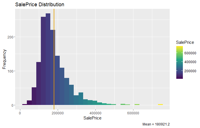
From the histogram above we can know that the SalePrice of most house distributed between 100000 - 300000. We can Further check relationships between variables and SalePrice.
# Kernel density plots
kit <- train[,c("KitchenQual", "SalePrice")]
lot <- train[,c("LotConfig", "SalePrice")]
sal <- train[,c("SaleType", "SalePrice")]
# SalePrice - KitchenQual
kit.plt <- ggplot(kit, aes(x = SalePrice, fill = KitchenQual)) +
geom_density(alpha = 0.4) +
labs(title = "SalePrice distribution by KitchenQual")
# SalePrice - LotConfig
lot.plt <- ggplot(lot, aes(x = SalePrice, fill = LotConfig)) +
geom_density(alpha = 0.4) +
labs(title = "SalePrice distribution by LotConfig")
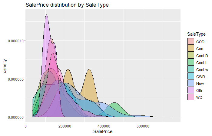
# SalePrice - SaleType
sal.plt <- ggplot(sal, aes(x = SalePrice, fill = SaleType)) +
geom_density(alpha = 0.4) +
labs(title = "SalePrice distribution by SaleType")
# Plot
kit.plt
lot.plt
sal.plt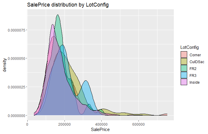
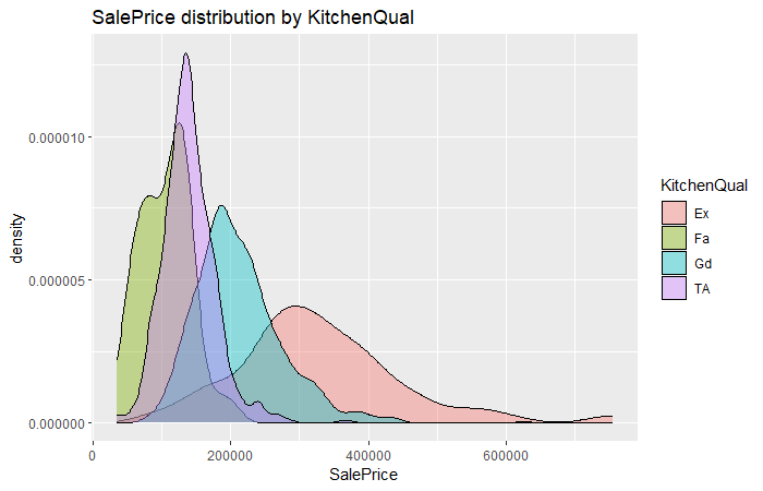
From these three density graphs presented above, we can see that the KitchenQual has pretty much influnce on SalePrice since there is an overt distinction performance on SalePrice between different level of KitchenQual.
On the contrary, the LotConfig almost does not affect SalePrice due to different level of LotConfig distributed similar on SalePrice.
For the thrid graph, it seems SaleType also has some effect on SalePrice, and we can comprehend further by checking its box plot.
# Boxplots
ggplot(sal, aes(x = SaleType, y = SalePrice, fill = SaleType)) +
  geom_boxplot() + labs(title = "SalePrice distribution by SaleType")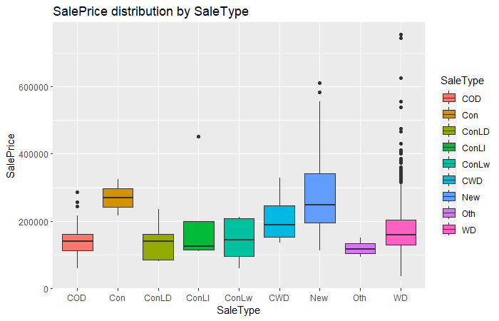
From the box plot presented above, we can clearly see that type "Con" has an obvious higher SalePrice than other SaleType.
Models
KNN
# Load library
library(caret)

# Set a seed
set.seed(123)

# Set up grid and trControl
grid_knn <- expand.grid(.k = seq(2, 20, by = 1))
tr.control <- trainControl(method = "cv")

# Fit a knn model
fit.knn <- train(
  SalePrice ~ .          ,
  data = train           ,
  method = "knn"         ,
  trControl = tr.control ,
  tuneGrid = grid_knn    ,
  preProcess = c("center", "scale")
)

# Present the model
fit.knn
Output:
## k-Nearest Neighbors
##
## 1460 samples
## 79 predictor
##
## Pre-processing: centered (259), scaled (259)
## Resampling: Cross-Validated (10 fold)
## Summary of sample sizes: 1312, 1313, 1315, 1316, 1314, 1315, ...
## Resampling results across tuning parameters:
##
## k RMSE Rsquared MAE
## 2 48308.97 0.6369849 29488.90
## 3 45175.54 0.6818478 27824.30
## 4 43468.41 0.7059687 26807.86
## 5 42229.03 0.7236226 25965.80
## 6 41517.57 0.7354519 25529.33
## 7 41532.49 0.7373131 25645.46
## 8 41254.27 0.7436025 25452.73
## 9 41064.91 0.7477132 25452.98
## 10 41350.02 0.7461180 25422.95
## 11 41348.11 0.7483068 25332.63
## 12 41360.71 0.7503443 25343.91
## 13 41281.48 0.7524483 25301.94
## 14 41291.97 0.7545341 25315.46
## 15 41187.60 0.7574072 25360.50
## 16 41222.73 0.7584467 25332.26
## 17 41429.09 0.7569665 25393.19
## 18 41399.33 0.7581937 25453.12
## 19 41415.85 0.7592843 25492.15
## 20 41409.30 0.7612812 25495.30
##
## RMSE was used to select the optimal model using the smallest value.
## The final value used for the model was k = 9.
# Visualize model
plot(fit.knn)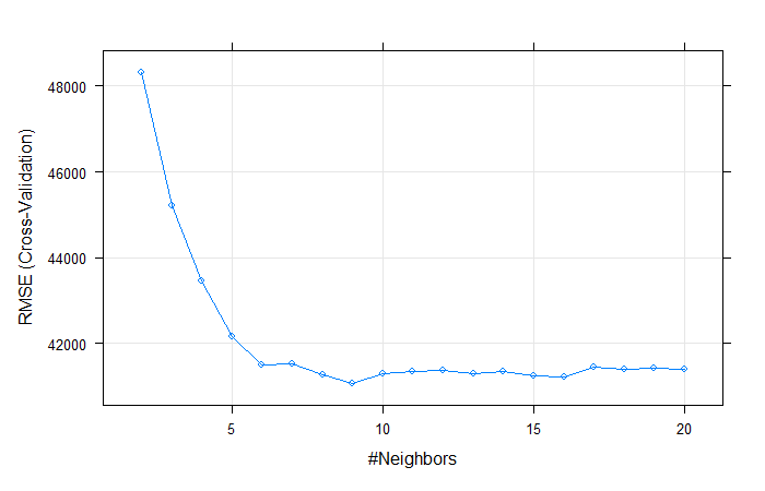
# Make prediction
pred.knn <- predict(fit.knn, newdata = test)

# Save prediction as knn.csv
write.csv(
  data.frame(Id, SalePrice = pred.knn),
  file = "knn.csv",
  row.names = FALSE
)
Linear Regression
Simple Linear Regression
# Fit a linear regression model
fit.lm <- lm(SalePrice ~ ., data = train)

# Visialize model
par(mfrow = c(2,2))
plot(fit.lm)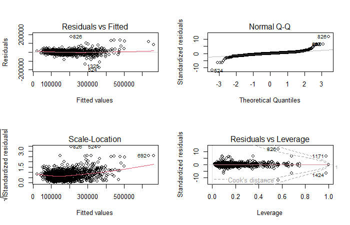
# Make prediction
pred.lm <- predict(fit.lm, newdata = test)

# Save prediction as lm.csv
write.csv(
  data.frame(Id, SalePrice = pred.lm),
  file = "lm.csv",
  row.names = FALSE
)
Linear Regression with Stepwise Selection
Forward
# Define empty and full
empty <- lm(log(SalePrice) ~ 1, data = train)
full  <- lm(log(SalePrice) ~ ., data = train)

# Fit a forward model
fit.forward <- step(
  empty,
  scope = list(lower = empty, upper = full),
  direction = "forward"
)

# Make prediction
pred.forward <- predict(fit.forward, newdata = test)

# Save prediction as forward.csv
write.csv(
  data.frame(Id, SalePrice = exp(pred.forward)),
  file = "forward.csv",
  row.names = FALSE
)
Backward
# Fit a backward model
fit.backward <- step(
  full,
  scope = list(lower = full, upper = empty),
  direction = "backward"
)

# Make prediction
pred.backward <- predict(fit.backward, newdata = test)

# Save prediction as forward.csv
write.csv(
  data.frame(Id, SalePrice = exp(pred.backward)),
  file = "backward.csv",
  row.names = FALSE
)
Shrinkage Methods
Ridge Regression
# Load library
library(glmnet)

# Set a seed
set.seed(123)

# Define x and y and lambdas
train.x <- train[,names(train) != "SalePrice"]
x <- data.matrix(train.x)
y <- log(train$SalePrice)
lambdas <- 10^seq(2, -3, by = -.1)

# Fit a ridge regression model
fit.ridge <- glmnet(
  x,
  y,
  alpha = 0,
  family = 'gaussian',
  lambda = lambdas
)
cv.ridge <- cv.glmnet(x, y, alpha = 0, nfold = 20, lambda = lambdas)

# Visualize model
plot(cv.ridge)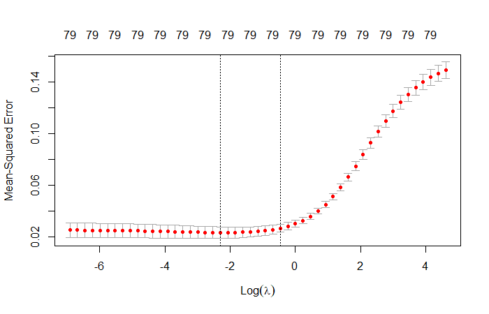
# Make prediction
pred.ridge <- as.vector(predict(
  fit.ridge,
  s = cv.ridge$lambda.min,
  newx = data.matrix(test)
))

# Save prediction as ridge.csv
write.csv(
  data.frame(Id, SalePrice = exp(pred.ridge)),
  file = "ridge.csv",
  row.names = FALSE
)
Lasso
# Fit a Lasso model
fit.lasso <- cv.glmnet(x, y, alpha = 1)
cv.lasso <- cv.glmnet(x, y, alpha = 1, nfolds = 10)

# Visualize model
plot(cv.lasso)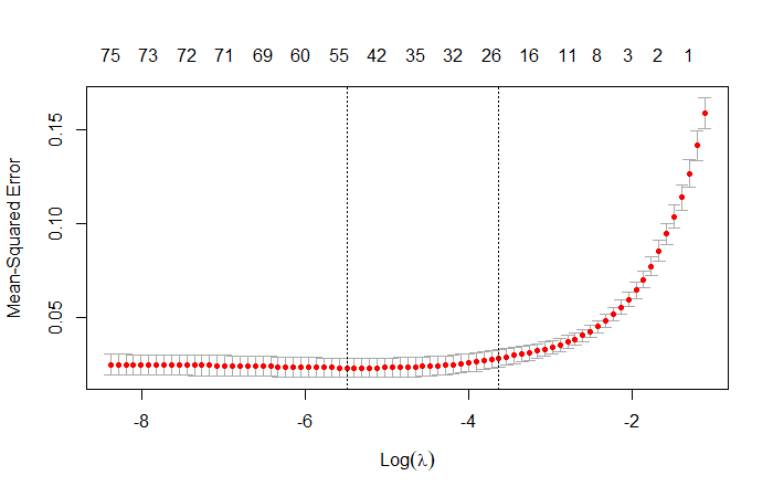
# Make prediction
pred.lasso <- as.vector(predict(
  fit.lasso,
  s = cv.lasso$lambda.min,
  newx = data.matrix(test)
))

# Save prediction as lasso.csv
write.csv(
  data.frame(Id, SalePrice = exp(pred.lasso)),
  file = "lasso.csv",
  row.names = FALSE
)
Generalized Additive Models
# Load libraries
library(splines)
library(gam)

# Fit a gam model
fit.gam <- gam(
  log(SalePrice) ~
  s(MSSubClass   , df = 5) + s(LotArea      , df = 5) +
  s(OverallQual  , df = 5) + s(OverallCond  , df = 5) +
  s(YearBuilt    , df = 5) + s(YearRemodAdd , df = 3) +
  s(MasVnrArea   , df = 5) + s(BsmtFinSF1   , df = 5) +
  s(BsmtFinSF2   , df = 5) + s(BsmtUnfSF    , df = 5) +
  s(X1stFlrSF    , df = 5) + s(X2ndFlrSF    , df = 5) +
  s(BsmtFullBath , df = 1) + s(FullBath     , df = 1) +
  s(BedroomAbvGr , df = 5) + s(KitchenAbvGr , df = 4) +
  s(TotRmsAbvGrd , df = 1) + s(Fireplaces   , df = 2) +
  s(GarageCars   , df = 2) + s(GarageArea   , df = 2) +
  s(WoodDeckSF   , df = 2) + s(ScreenPorch  , df = 4) +
  s(PoolArea     , df = 5) + s(MoSold       , df = 1) ,
  data = train
)

# Make prediction
pred.gam <- predict(fit.gam, newdata = test)

# Save prediction as gam.csv
write.csv(
  data.frame(Id, SalePrice = exp(pred.gam)),
  file = "gam.csv",
  row.names = FALSE
)
Regression Trees
# Load libraries
library(MASS)
library(rpart)
library(rpart.plot)

# Fit a tree model
fit.tree <- rpart(log(SalePrice) ~ ., data = train)

# Visualize model
rpart.plot(fit.tree)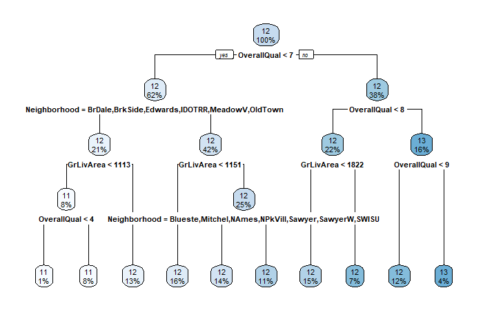
# Make prediction
pred.tree <- predict(fit.tree, test)

# Save prediction as tree.csv
write.csv(
  data.frame(Id, SalePrice = exp(pred.tree)),
  file = "tree.csv",
  row.names = FALSE
)
Bagging
# Set a new trControl
tr.control <- trainControl(
  method = "repeatedcv" ,
  number = 10           ,
  repeats = 10
)

# Fit a bag model
fit.bag <- train(
  log(SalePrice) ~ .     ,
  data = train           ,
  method = "treebag"     ,
  trControl = tr.control ,
  control = rpart.control(minsplit = 2, cp = 0)
)

# Check model
fit.bag
Output:
## Bagged CART
##
## 1460 samples
## 79 predictor
##
## No pre-processing
## Resampling: Cross-Validated (10 fold, repeated 10 times)
## Summary of sample sizes: 1314, 1312, 1316, 1313, 1314, 1315, ...
## Resampling results:
##
## RMSE Rsquared MAE
## 0.1461835 0.8677392 0.09949275
# Make prediction
pred.bag <- predict(fit.bag, newdata = test)
# Save prediction as bag.csv
write.csv(
data.frame(Id, SalePrice = exp(pred.bag)),
file = "bag.csv",
row.names = FALSE
)
Random Forest
# Set up grid for random forest
grid_rf = expand.grid(.mtry = c(2, 4, 8, 16, 32, 64))

# Fit a random forest model
fit.rf <- train(
  log(SalePrice) ~ .     ,
  data = train           ,
  method = 'rf'          ,
  trControl = tr.control ,
  tuneGrid = grid_rf
)

# Check model
fit.rf
Output:
## Random Forest
##
## 1460 samples
## 79 predictor
##
## No pre-processing
## Resampling: Cross-Validated (10 fold, repeated 10 times)
## Summary of sample sizes: 1314, 1314, 1313, 1314, 1315, 1314, ...
## Resampling results across tuning parameters:
##
## mtry RMSE Rsquared MAE
## 2 0.2224998 0.8110924 0.15557015
## 4 0.1754462 0.8496995 0.11851156
## 8 0.1541188 0.8717045 0.10210873
## 16 0.1447798 0.8810869 0.09554608
## 32 0.1397476 0.8858131 0.09231193
## 64 0.1377846 0.8864992 0.09126339
##
## RMSE was used to select the optimal model using the smallest value.
## The final value used for the model was mtry = 64.
# Visualize model
plot(fit.rf)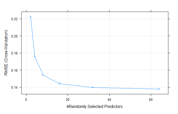
# Make prediction
pred.rf <- predict(fit.rf, newdata = test)

# Save prediction as rf.csv
write.csv(
  data.frame(Id, SalePrice = exp(pred.rf)),
  file = "rf.csv",
  row.names = FALSE
)
Boosting model
# Load library
library(gbm)
set.seed(123)

# Fit a model
fit.gbm <- gbm(
  log(SalePrice) ~ .        ,
  data = train              ,
  distribution = "gaussian" ,
  interaction.depth = 4     ,
  shrinkage = 0.01          ,
  n.tree = 5000             ,
  cv.folds = 20
)

# Make prediction
pred.gbm <- predict(
  fit.gbm,
  newdata = test,
  n.trees = which.min(fit.gbm$cv.error)
)

# Save prediction as gbm.csv
write.csv(
  data.frame(Id, SalePrice = exp(pred.gbm)),
  file = "gbm.csv",
  row.names = FALSE
)
Prediction
Ensemble
For the final prediction, I choose 3 models with highest grades to build an ensemble model. Since this is a regression problem, I decided to use the weighted average of their prediction as the final prediction.
# Make prediction
prediction <- ((exp(pred.gbm)*7) + (exp(pred.gam)*2) + (exp(pred.lasso)*1))/10

# Save prediction as prediction.csv
write.csv(
  data.frame(Id, SalePrice = prediction),
  file = "prediction.csv",
  row.names = FALSE
)